2. First Steps
First steps into AthosGEO View are basically first steps into ParaView, because it is most important to understand the underlying logic of sources, filters, viewers and more. Understanding this logic will give you the ability to find solutions for problems that are not covered in any user’s manual or documentation on your own, while the same thing may be extemely difficult if you are looking for solutions that resemble those with other softwares that you may know already.
Anyway, humans tend to be impatient, and being sent to learning ParaView first instead of going directly into the applications that are of immediate interest is an advice that not many people will be ready to follow. For this reason, the following section will show how to visualize a first built-in block model example, just to give you an impression.
But then you will find a section that will show you the entry point to a step by step introduction - starting with learning the basics of ParaView.
If even this cannot convince you to take one step after the other, a third section will give you at least some few hints about the most basic concepts of ParaView and AthosGEO View.
2.1. A First Impression
Once the AthosGEO View software is installed and started, a demo model can be opened very easily through the Help menu: Selecting Example Cases will open a dialog as shown in Fig. 2.1, with the choice of two possible example visualizations.

Fig. 2.1 A choice of two example visualizations are built into an installed AthosGEO View software
2.1.1. First Demo Example
The first example shows a demo block model, together with a background topography and aerial photo, as can be seen in Fig. 2.2.
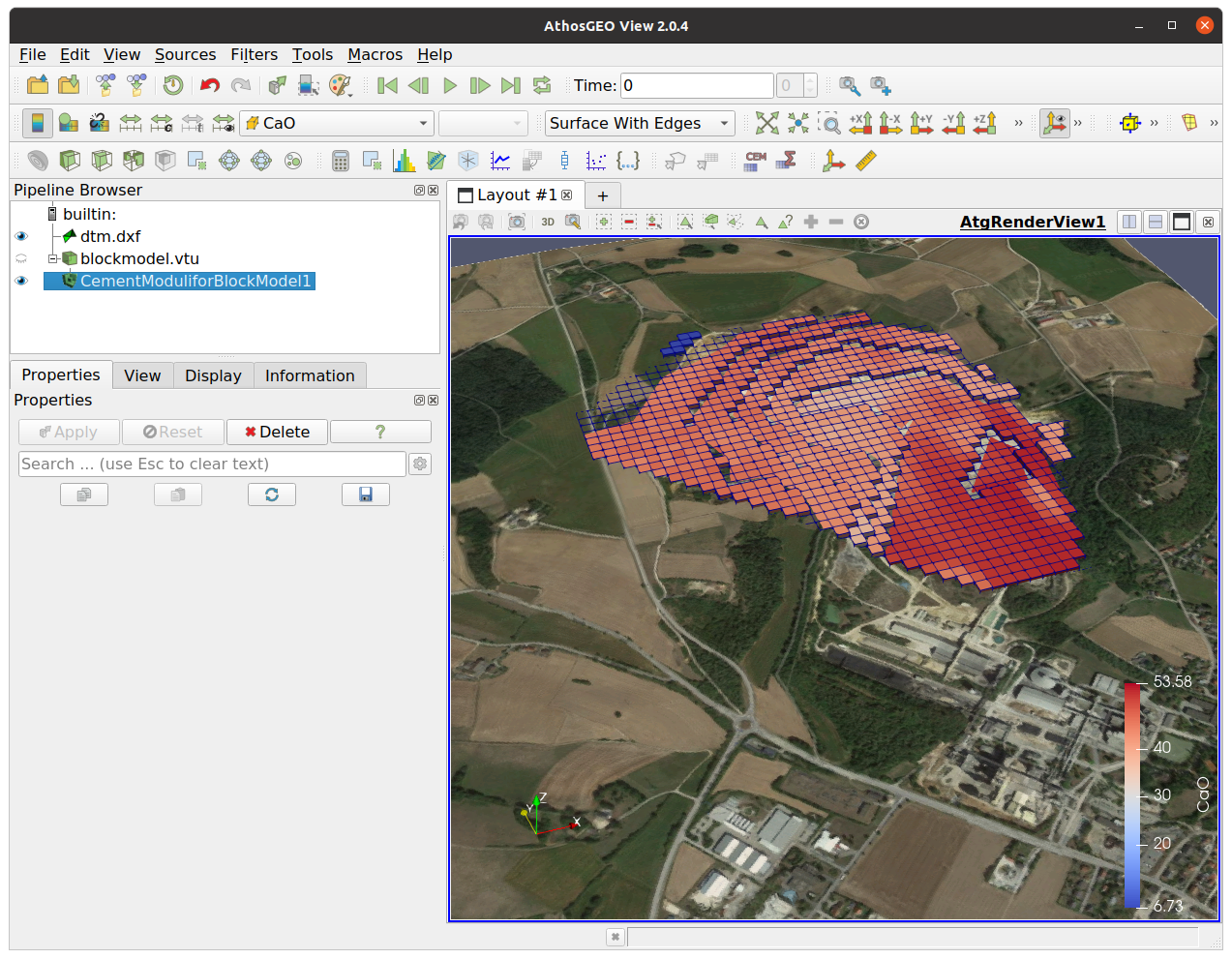
Fig. 2.2 Display of Demo model display with topography and aerial photo as a background.
2.1.2. The Render View
At the right side of the screen, in the view area, an Athos Render View shows a 3D display of the block model, together with a topography, that can be zoomed in and out, rotated and panned (moved) with the mouse interactively.
The blocks of the model are colored according to their content of CaO.
2.1.3. The Pipeline Browser
The Pipeline Browser is found at the upper left side of the view area. It shows the different data objects together with their relations. At the left side of the different items, an eye symbol is shown if the item can be displayed in the currently active view. Clicking on that eye will toggle it between open and closed, which toggles between showing and hiding the respective item.
Clicking on an item directly will make it active. Once a pipeline item is active, some view parameters can be adapted in the different combo boxes in the toolbar (see Fig. 2.3):
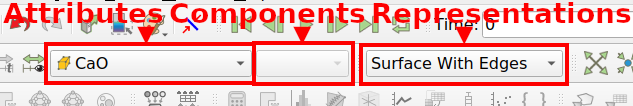
Fig. 2.3 The Tool Bar Combo Boxes are always referring to the active pipeline item in the current active view
In the Attributes combo box, an attribute can be selected for coloring of the blocks in the model.
The Components combo box is for attributes with several components, like a coordinate that has 3 components for the X, Y and Z direction.
The Representations combo box allows to select a representation for a pipeline item, like Surface, Surface with Edges, Feature Edges and others.
2.1.4. The Properties Panel
The Properties Panel is at the lower left of the screen in the default configuration (which can be easily changed by the user). It comes with the following four tabs:
Properties
This tab allows to manage available properties of the currently active pipeline item. After doing some change, the user needs to press Apply to apply the changes.
View
The View tab is about properties of the current view, thus referring not only to one single pipeline item, but to the entire view. An example would be the display of coordinate axes. Changes will be applied immediately, without the need to explicitly press Apply.
Display
The Dislay tab refers to the representation of a currently active pipeline item within the current view. In the example it would apply e.g. to the block model, but not to the topo surface. Also the Display properties are immediately applied without further user action.
Information
This tab is of interest if the user wants to see what are the actual data items corresponding to the currently active pipeline item. This is for information purposes only, nothing to be changed by the user.
Did you know?
Like many other dialog windows within AthosGEO View, all these panels have a
normal and an advanced mode that may show some less commonly used
properties, and pressing the  button in the upper right
part of the panels toggles between the two modes.
button in the upper right
part of the panels toggles between the two modes.
To the left of this button, there is also a Search entry field that assists with the management of large and sometimes a bit confusing panels: Just start typing the first letters of a property that you are looking for, and all properties that do not start with these letters will automatically be hidden.
2.1.5. Second Demo Example
The second example that is accessible through the Example Cases dialog in Fig. 2.1 is about different view types as shown in Fig. 2.4.
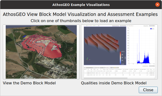
Fig. 2.4 This example shows 4 different ways to display the data of a block model
This second example shows several different ways to visualize the data of a block model:
In the Athos Render View, the complete block model (blockmodel.vtu in the pipeline browser is displayed with a Volume View representation. This is a display where the blocks are not only colored, but have also a transparency assigned to it, with the highest values not only in red, but also with the highest opacity. This is a way how for example lenses of material with a higher content of some chemical compound can be visualized even “inside” the block model.
In the same Athos Render View, the block model is visualized a second time, but after having cut into a series of slices by using the Slice Filter that is also visible in the pipeline browser.
At the bottom of the view area, the same block model is displayed in a Athos Summary View. This is a tabular view where all the attributes are summarized according to their specific account type: tonnages are simply added, chemical compounds are tonnage weighted mean values of the entire model, etc.
At the right side of the view area, a Histogram View shows the distribution of CaO contents in the block model. With the Display properties panel it is possible to select another attribute or chemical compound for display and adapt the number of bins.
2.2. Start with ParaView
After these first impressions from the example cases, it may be worth understanding the basic concepts of the AthosGEO View software a bit more, which happen to be the same as those of ParaView. For this reason it is recommended that you continue now with an introduction into ParaView for which you find an introduction here:
https://docs.paraview.org/en/latest/
Most of the things that are described in the ParaView documentation can be directly applied also in AthosGEO View. The easiest way to get also access to the ParaView example cases is an installation of that software which is described in the documentation.
Note
Some features from ParaView were disabled in AthosGEO View in order not to overload that software with features that are not applicable for geodata visualizations.
The ParaView documentation is not only of interest for the basic concepts, but also for more detailed information about advanced features like the Python support which exists also in AthosGEO View but not handled in this current documentation.
2.3. For Those who Cannot Wait
2.3.1. Pipeline Elements
With the VTK, data processing always works along a pipeline of filters, with filters being any kind of data processing module, as symbolized in Fig. 2.5. The power of this approach is it’s enormous flexibility because filters can be added or removed at any time.

Fig. 2.5 The VTK data processing filter pipeline
ParaView and with it also AthosGEO View are visualizing this abstract concept in the Pipeline Browser that allows the user to add, remove or reconnect the filters within the pipeline.
So basically the elements of the pipeline are filters in general, with input and output pipes, but there are also special cases of filters:
Sources
These are filters without an input pipe because they are generating data from scratch. An example would be the Sphere filter that generates the geometry of a sphere with a specified center location and radius.
Readers
These are also filters without an input pipe because they are reading their input from a disk file.
Writers
As counterparts of the readers, these have no output pipe, bit instead they are writing the data into a disk file. Writers do not appear in the pipeline, but they are called with the Save Data command.
Views
Also the views are considered filters without an output pipe. Also they are not symbolized in the Pipeline Browser, but instead they are generating screen output either graphically or in tabular form.
Extractors
A new type of pipeline items are the Extractors (since ParaView version 5.9). They can be inserted into the pipeline in order to extract intermediate data on request and write them to files.
Summarizing, Pipeline Items as visualized in the Pipeline Browser can be considered as being Filters in the sense of the VTK, because by choosing a filter (or source) from the ParaView main menu will result in adding a corresponding icon.
But if you want, you can also consider them as representing the data output of a filter that can be analyzed by looking at the Information panel, written to a file or visualized in a view.
Did you know?
Online help for all the available filters, sources, readers and writers is available through the Help menu through the Filter, Reader and Writer Reference command. Find there a short description of the purpose, together with input, output and properties of all the filters.
2.3.2. Data and State Files
The Save Data command (or  from the toolbar) will save
the output data of the currently active pipeline item to a data file.
from the toolbar) will save
the output data of the currently active pipeline item to a data file.
The Save State (or  ) will write a *.pvsm file that
describes the current state of the pipeline, meaning: the filters with
their properties and connections. However, it does not write the
data that were loaded from disk files.
) will write a *.pvsm file that
describes the current state of the pipeline, meaning: the filters with
their properties and connections. However, it does not write the
data that were loaded from disk files.
Did you know?
A state file contains also the full file names of the data files that are part of the current state of the pipeline (because these are actually properties of the readers), but sometimes it happens that these paths are not any more correct, like after moving data and state files to another computer. This is not a problem with AthosGEO View because on reading a state file, the program will ask whether to keep the current paths, look for all the files in a different path, or specify the correct path for each single data input file.
2.3.3. Points and Cells
When dealing with VTK type 3D geometries it is good to know that they are made up of points and cells that are in a way independent. Let’s take a little triangulated surface as an example as shown in Fig. 2.6.
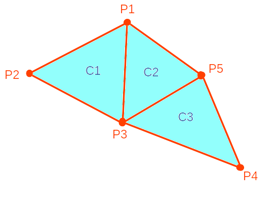
Fig. 2.6 A little triangulated surface, made up of 5 points and 3 cells of type triangle
Data of this little example will be stored in two tables, as shown in Table 2.1 and Table 2.2.
PointID |
X |
Y |
Z |
|---|---|---|---|
1 |
x1 |
y1 |
z1 |
2 |
x2 |
y2 |
z2 |
3 |
x3 |
y3 |
z3 |
4 |
x4 |
y4 |
z4 |
5 |
x5 |
y5 |
z5 |
CellID |
CellType |
Points |
|---|---|---|
1 |
triangle |
1, 3, 2 |
2 |
triangle |
5, 3, 1 |
3 |
triangle |
4, 3, 5 |
In the case of a block model, cells are of type hexahedron, defined by 8 points. This knowledge about points and cells helps to better understand the following section.
2.3.4. Point, Cell, Field and Row Data
Geometries in VTK can have attached attributes of several different types:
Point Data
A table of data, with each data row assigned to a point.
Cell Data
A table of data, with each data row assigned to a cell.
Field Data
A table of data, with the rows not assigned to anything special.
In addition to these data types, there are still the
Row Data
These are basically tables of data which are not assigned to any geometry.
2.3.5. And Once More…
For more detailed and thorough information about all the concepts that were shortly introduced here please refer to the ParaView documentation as explained here in Section 2.2.