7. Surfaces and Lines
Besides the visualization of block models and sampling sets, AthosGEO View is able to visualize all kinds of geometric items that also ParaView would handle. For the purpose of geodata visualization, it is often desirable to add items like:
Topography, including a projected aearial photo, a geological map, a topographic map or any other kind of mapping.
Boundary lines (closed polylines) like lease or any other aereal boundary, or any kind of other polylines showing important features.
Note
The following will give only a small impression of the possibilities to show additional geometries with AthosGEO View. Please have a look into the ParaView documentations for further instructions: First Steps.
7.1. Triangulated Surfaces
7.1.1. Reading from File
The native file format for triangulated surfaces in VTK is a polydata file (with .vtp extension). With AthosGEO View comes the additional possibility to read them also from .dxf files, and from ParaView comes the ability to read even more formats.
7.1.2. Reading from GeoTIFF File
AthosGEO View is able to read a topography from a TIFF file if it contains rastered altitude values in GeoTIFF format.
The displayed output will be a triangulated surface that is automatically generated and optionally reduced (decimated) from the input raster data.
Regarding the reduction options see Section 7.1.4.
7.1.3. Generating from Points
If a series of surface point coordinates (x, y, z) are available, a surface can be triangulated between them with AthosGEO View. The starting point could be a CSV file with a table like in Table 7.1.
x |
y |
z |
|---|---|---|
10200 |
24300 |
190 |
10200 |
24310 |
192 |
10200 |
24320 |
195 |
10200 |
24330 |
199 |
10200 |
24340 |
205 |
10200 |
24350 |
212 |
10200 |
24360 |
215 |
10200 |
24370 |
217 |
10200 |
24380 |
218 |
10200 |
24390 |
217 |
10200 |
24400 |
214 |
10210 |
24300 |
191 |
10210 |
24310 |
192 |
etc. |
In AthosGEO View, open the points CSV file and choose the CSV Reader for loading the data into a table as in Fig. 7.1.
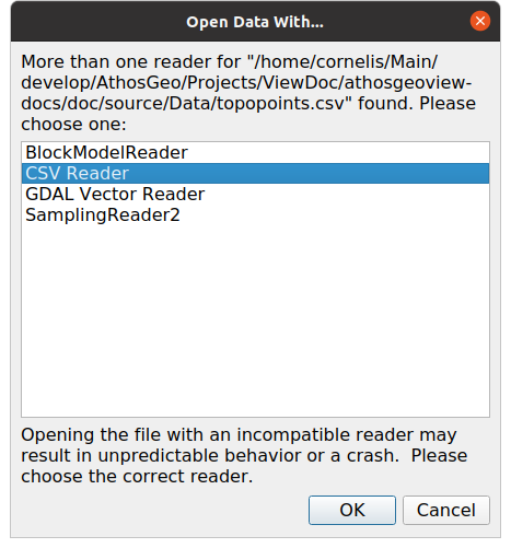
Fig. 7.1 The CSV Reader reads a CSV file and displays it as a table in a SpreadSheet View.
On pressing Apply, a SpreadSheet View will open and show the points table as in Fig. 7.2.
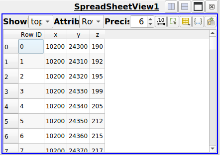
Fig. 7.2 Point coordinates displayed in a SpreadSheet View.
Next, these tabular data need to be converted into geometric points in space by applying the Table to Points filter.
Did you know?
A quick way to get that Table to Points filter is through Filters → Search… and starting to type the word Table: The filter will immediately appear in the list and with a click and pressing Enter it is attached to the filter pipeline.
In the appearing Properties panel of the Table to Points filter, table columns for the x, y and z coordinates need to be specified, see Fig. 7.3.
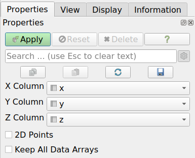
Fig. 7.3 The Properties panel of the Tables to Points filter.
Hint
Before pressing Apply, make sure that a render view (3D view) is activated: Only then you will see the new points immediately, while otherwise they will be displayed in the SpreadSheet View that was previously showing the table data.
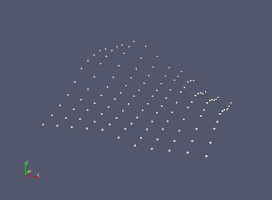
Fig. 7.4 Display of points in an AthosGEO Table View.
With this we have free points in space as shown in Fig. 7.4 and the next step would be to triangulate a topo surface between them using the Delaunay 2D filter.
Note
Two other filters look like they would do the same or similar things, but this is not true:
The Triangulate filter does not triangulate a surfass between points, but converts surfaces that are made up of face elements (cells) that are more complex than simple triangles (like quads, polygons or triangle strips) into plain triangulated surfaces. This is a requirement for certain other filters that cannot handle these more complex surface elements.
The Delaunay 3D filter might look like the adequate filter for our purpose, because we want to generate a surface in 3D space. However, This filter actually does not generate triangles, but tetrahedra, filling the void space inside a shell.
The Properties of the Delaunay 2D filter is shown in Fig. 7.5. xx
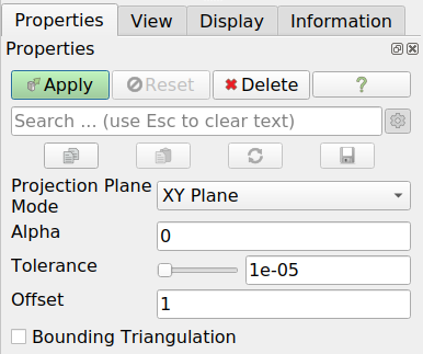
Fig. 7.5 The Properties panel of the Delaunay 2D filter that will triangulate a surface between a set of points.
Select the XY Plane option for generating a topo surface.
The Tolerance is the distance between points below which are considered identical and merged. For a topo with coordinates in meters, the default value might be too small, so better increase it to something like 0.01.
After pressing Apply, a surface will appear as shown in Fig. 7.6.
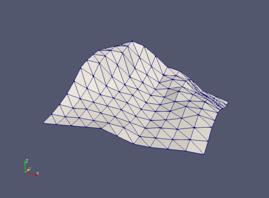
Fig. 7.6 A triangulated surface generated from input points using the Delaunay 2D filter.
At this point, a new triangulated surface is often too finegrained, with too many points and triangles to best represent the topo surface. A clever way to reduce the number of triangles in order to optimize the representation is described in Section 7.1.4.
7.1.4. Reduction of Triangulated Surfaces
The Decimate filter (to be found at Filters → Geometry) allows to reduce the number of triangles in a triangulated surface in an intelligent way, preserving morphologic features as much as possible within the limits of the selected parameters, see Fig. 7.7.
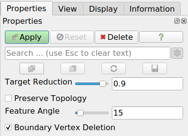
Fig. 7.7 The Properties panel of the Decimate filter allow to finetune the resulting output triangulation.
Did you know?
The Decimate filter works only for surfaces that are plain triangulated surfaces without any other surface elements, like quads, polygons etc. If this is not true for a given surface, the Triangulate filter needs to be applied first.
The two most important Properties of the Decimate filter are:
Target Reduction: A value of 0.9 means that the number of triangles should be reduced by 90% if this is possible while respecting the other constraints of the reduction. If the reduction looks too extreme, reduce this value to retain more triangles.
Feature Angle: Any common edge between two triangles where the angle between the triangles is more than the feature angle, must not be removed. So if the result of a decimation looks like retaining morphologic features not good enough, reduce that angle, or vice versa.
Example: The result of reducing the surface shown in Fig. 7.6 with the Decimate filter default properties as shown in Fig. 7.7 will produce a result as shown in Fig. 7.8. Visually, a much less radical reduction with Target Reduction of only 0.3 and a Feature Angle of 10 seems to generate a better result, as shown in Fig. 7.9.
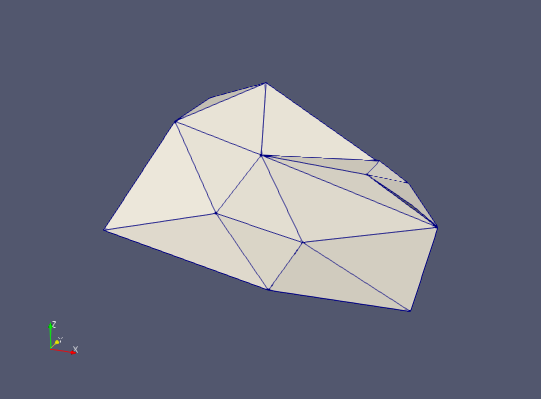
Fig. 7.8 The surface shown in Fig. 7.6 after application of the Decimate filter with default properties.
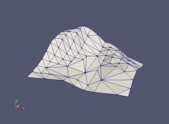
Fig. 7.9 The surface shown in Fig. 7.6 after application of the Decimate filter with a much more optimum set of properties (Target Reduction = 0.3, Feature Angle = 10).
The optimum set of properties for the Decimate filter will depend on the input triangulated surface and the requirements of retaining morphologic features with higher or lower precision.
7.1.5. Reduction of Polylines
The Decimate Polyline filter will reduce the number of points definint a polyline in such a way that the geometry will be affected as little as possible.
7.1.6. Writing Triangulated Surfaces and Polylines
The native VTK format for triangulated surfaces and polylines is a Polydata File, with .vtp extension.
Writing them to .dxf file is an extension of AthosGEO View to allow data exchange with softwares that prefer such a format.
A number of other formats are already supported by ParaView.
7.2. Projected Maps
7.2.1. Georeferencing
Topo surfaces are having coordinates from their points, but images with maps or aerial photos need to be xplicitly georeferenced in order to be correctly projected onto a topo. Two systems are recognized in AthosGEO View:
ESRI worldfiles are small plain text files describing the positioning of the image relative to a geographical reference grid. If they exist, AthosGEO View will find and use them.x
In the case of GeoTIFF, the georeferencing information is incorporated within the image file itself. If a TIFF image file contains such information, AthosGEO View will use it.
7.2.2. The Texture Georeferenced Filter  
The Texture Georeferenced filter asks for the name of a georeferenced texture (image) file, as specified above.
Next, select the Topo with Map Texture representation, instead of the common Surface or Surface with Edges representations.
The example topo with a projected example map Fig. 7.10 would look like shown in Fig. 7.11.
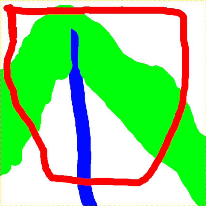
Fig. 7.10 The map to be projected on the topo¶ |
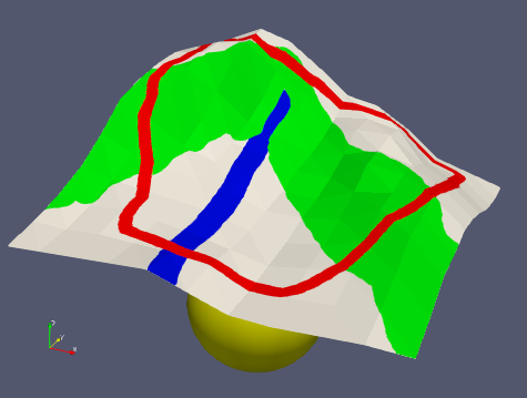
Fig. 7.11 An example topo with the projected example map.¶ |
Hints
The Texture Georeferenced filter actually adds the full texture file name and path to the Field Data of the triangulated surface (topo). That means, if the output of that filter would be saved to a *.vtp file, also that texture file name will be saved.
If now that *.vtp file is loaded back to AthosGEO View, if the representation is then switched again to Topo with Map Texture, and if finally the texture file is still present in the same path, the topo projection will be back even without applying the Texture Georeferenced filter again.
7.2.3. Textures with Transparency
By default, the Ignore Alpha property of the Texture Georeferenced is on, meaning: If a texture map file has an alpha channel, care will be taken that the entire texture map is interpreted as being opaque.
If that property is off, an alpha channel will be respected, with dramatic effects: It does not only affect texturing of the topo surface, but it makes the topo surface itself fully or partially transparent.
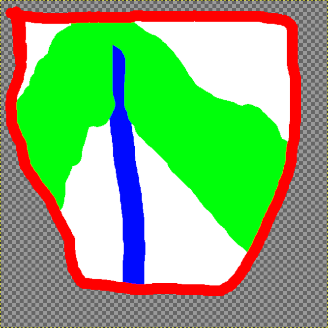
Fig. 7.12 This example map is fully transparent in the areas that are not of interest¶ |
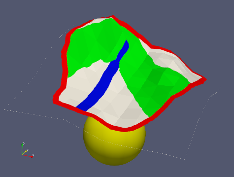
Fig. 7.13 The effect is like clipping the topo along the boundary of the range of interest¶ |
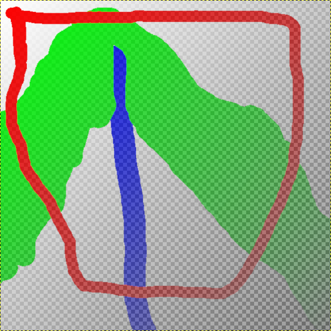
Fig. 7.14 This example map has a transparency gradient from the upper left to the lower right corner¶ |
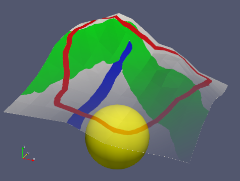
Fig. 7.15 The effect is a textured topo surface with varying transparency (The underlying sphere becomes increasingly visible)¶ |
7.3. Lines, Polylines and Polygons
7.3.1. Reading from File
The native file format for lines, polylines and polygons in VTK is a polydata file (with .vtp extension). With AthosGEO View comes the additional possibility to read them also from .dxf files, and from ParaView comes the ability to read even more formats.
7.3.2. Manually Generating Polylines or Polygons
With AthosGEO View it is possible to manually digitize lines, polylines and polygons using the Poly Line Source. It can be found at Sources → Geometric Shapes. With this, a Properties panel will appear as shown in Fig. 7.16.
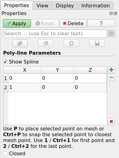
Fig. 7.16 The Poly Line Source Properties panel explains the different steps to manually digitize a polyline. If the Closed checkbox is checked, the polyline will be automatically closed, generating a polygon. With the +, - and x buttons, single points can be added or removed, or the entire list will be cleared.
With a map in the background, a drawn polygon can be digitized as a geometric polygon object for further processing or activities, as shown in Fig. 7.17.
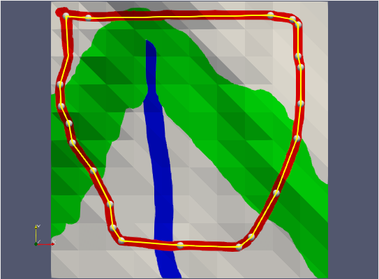
Fig. 7.17 The yellow spline was manually adapted to the red outline in the example map.
Hints
Make sure that the projection is parallel, and this can be achieved by unchecking the Camera Parallel Projection checkbox in the View panel.
Make sure that the view is exactly vertical, which can be achieved by pressing the -Z button in the toolbar.
It is possible that the spline disappears behind the topo surface because the Z coordinate is too low. It is not possible to directly change the Z coordinate in the Properties panel, so some tricks need to be applied. One possibility:
After activating the Poly Line Source and ensuring the parallel projection, rotate to a side view, e.g. by pressing +Y in the tool bar.
Move the mouse to the highest point in the model (maybe a zoom in is required for the precision) and press both the 1 and the 2 buttons, one after the other, in order to bring both the start and the end point to that elevation.
Press the -Z button to change to the top view. Start and end point are now coinciding, but visible, at the highest possible elevation.
Now move the start and end points to where they should be: the Z coordinate will remain at the elevation of the top point of the topo, and the same is true for all points that are added from now on.
At the end, do not forget to press the Apply button, because the spline that can be manipulated with with the mouse, is not yet the geometric object (polyline, polygon) that can be visualized, saved or otherwise further processed.