3. Display Table (and other) Data¶

The AthosGEO View program inherits abilities to display and analyze tabular data from the ParaView software. Tabular data can be read directly from CSV Files, but also the attributes of geometric objects are basically tabular data and the following explanations apply to them as well.

Did you know?

For geodata processing with AthosGEO View the most important geometric objects are one of the two VTK data types:

Unstructured Grid (block models, sampling sets) and
Poly Data (surfaces and polylines, both closed or open, as well as point sets).

These data objects are made up of two elements that are internally kept separate (which makes data manipulation much more efficient):

Points with their coordinates
Cells that are everything else: triangles in the case of a triangulated surface, line segments in the case of polylines, hexahedra in the case of block models or many other 3D elements in the case of sampling sets. These cells have no coordinates, but refer via internal ID numbers to the points.

On top of that, all these data elements can be connected with attribute data, which are basically all data tables:

Point Data are attached to the points. The point data table has the same number of rows as the point data set has points, so one data row refers to exactly one point. The number of columns is free, and the data types of the columns can be all different, numeric or strings.
Cell Data are attached to the cells, and each cell is again related to one row in the cell data table. Block model attributes are actually cell data.
Field Data are data tables that are attached to the entire data object, without a relation to single points or cells.

All the above tabular data are included in the following explanations about display and management of table data. One additional data table type is

Row Data which are data tables that are not related to any geometric objects, possily read directly from a CSV File.

Note: This explanation of VTK data object types, points, cells etc. is by far not exhaustive. For more detailled information see: VTK File Formats.

3.1. Table Views¶

The most simple display for table data is one of the two available table views (see Fig. 3.9).

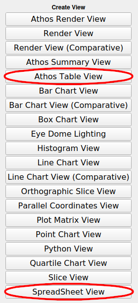
Fig. 3.9 Both the Athos Table View and the SpreadSheet View can display tabular data in a table format. The first is derived from the latter, and the difference is only the ordering of the columns.¶

These are the available table views in AthosGEO View:

SpreadSheet View

This table view does not really offer the functionality of a spreadsheet, but shows the content of a data table in tabular form, including numeric and string data. By default, the Point Data of a geometric data object are shown, so for a block model or a sampling set, the display has to be manually switched to Cell Data: see Fig. 3.10. A plain table like it can be read from a CSV File is shown as Row Data.

Athos Table View

This table view is derived from the SpreadSheet View and only the ordering of the columns is different: While the first orders the columns alphabetically, this view is tailor made for the needs of displaying block model and sampling set data in a more clearly arranged way for that purpose, as can be seen in Fig. 3.11. One more detail: The default display on opening an Athos Table View is Cell Data because only with this the user will see the data content of a block model or sampling set directly.

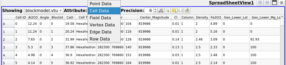
Fig. 3.10 The SpreadSheet View is the table view of ParaView. Please note the little buttons above the header line of the table: They allow to specify the number of displayed digits, switch between scientific and fixed point notation, show or hide table columns and either all rows or selected rows only and finally write the table data to a CSV file.¶

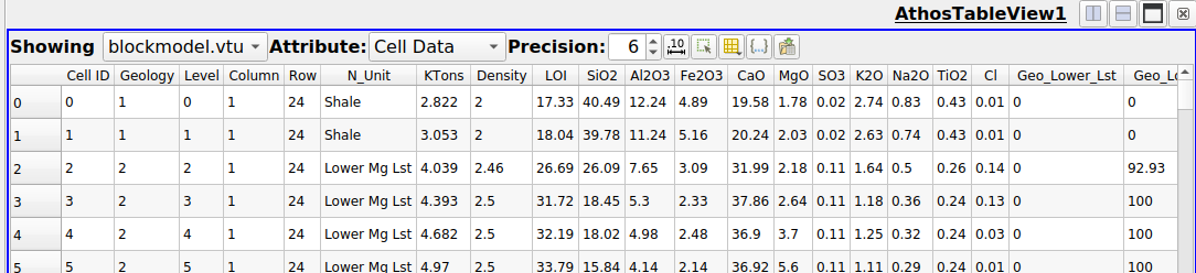
Fig. 3.11 The Athos Table View shows first the category columns, followed by tonnages and chemical compounds and others. All the other functionality is inherited from the SpreadSheet View.¶

3.1.1. CSV Reader for Athos Table View¶

Opening a CSV file will first open a reader selection dialog (see Fig. 3.12).

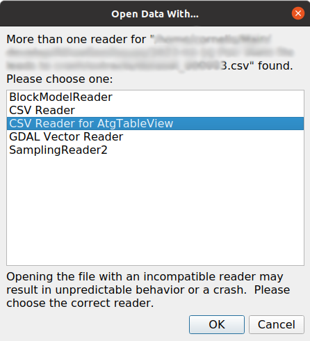
Fig. 3.12 Choice of readers for CSV files¶

Both the CSV Reader and the CSV Reader for Athos Table View will interpret CSV files as simple tables and display them accordingly:

The CSV Reader will display the file in a SpreadSheet View
The CSV Reader for Athos Table View will display the same file in an Athos Table View

3.1.2. Table Tool Buttons¶

At the upper right of an Athos Table View there is a little toolbar (see Fig. 3.13), with the following functionality:

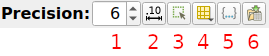
Fig. 3.13 The Athos Table View tool bar buttons. They are the same as for the Athos Summary View (see next section).¶

Precision: enter the number of valid digits in the numeric output
Representation: scientific or fixed point
Show either all or only selected elements
Choose the columns to display in the table
Cell connectivity is not being used for AthosGEO View
The Export Spreadsheet function allows to write the currently shown table content to a CSV file. The difference to the Save Data function is the fact that it maintains column order and other display settings, while the latter always writes the entire table to a file.

3.2. Summary Tables¶

Summarizing quality data from block models means calculating tonnage weighted means of the quality attributes. However, other attributes require a different handling, and this is one of the main reasons for the introduction of the different attribute categories in AthosGEO View - see Attribute Conventions.

The display of a data table with the Athos Summary Table will result in an automatically summarized display of the data as shown in Fig. 3.14.

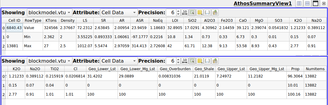
Fig. 3.14 Athos Summary View display of the same data as in Fig. 3.11.¶

The Athos Summary View shows 3 rows of data, as indicated in the Row Type column:

Value:
The calculated summary value for a specific attribute.

Min:
The lowest value of a specific attribute within the range of the summary.

Max:
The highest value of a specific attribute within the range of the summary.

The applied operations for the different attribute categories are summarized in Table 3.2.

Table 3.2 Summarizing *operations* for different *attribute categories*¶
Attribute Category	Examples	Summarizing Operation
Direct	SiO2, CaO	Tonnage weighted means
Derived	LS, SR, AR	Recalculate from tonnage weighted means
Tonnage	KTons, Taken	Sum
Weight	Pit, Zone	Tonnage weighted means
Category	Code, Level	Skip
SpecTonnage	Density	Volume weighted means
Others	coordinates, block sizes	Skip

A number of properties can be adapted for the Athos Summary View, and this can be done in the Display tab as shown in Fig. 3.15.

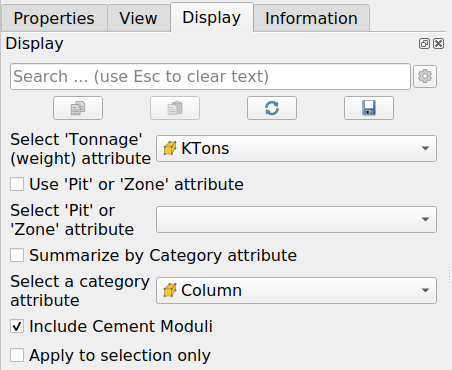
../_images/athossummaryview_properties.png

Fig. 3.15 Properties of the Athos Summary View can be adapted in the Display panel.¶

The following properties can be changed:

Tonnage Attribute

Every block of a block model must have at least one Tonnage type attribute, either Tons or KTons. But it is possible to have additional tonnages like Taken, which is the tonnage that was taken for a specific planning and which can be less than the total tonnage if only part of the block is required for the planning. If now the total taken tonnage is needed, Taken should be selected here.

Pit or Zone Attribute

In order to ignore all the tonnages outside of a specific pit or zone, it can be selected here. Do not forget to check the check box to make it happen.

Summarize by Category Attribute

Normally the summary table has exactly the 3 rows as explained in Fig. 3.14. However, if Summarize by Category attribute is on, for each existing value of the selected Category such a row triple will be calculated.

Include Cement Moduli

No matter if the input table had cement moduli or not, the output will have them calculated if this option is checked.

Apply to Selection Only

With this it is possible to select a number of blocks and automatically calculate the summary for these blocks only. If blocks are unselected or blocks added to the selection, the Athos Summary View will be updated on the fly.

Did you know?

Besides the Athos Summary View, summarizing of tabular data can also be done with the Summarize Attributes filter. Two things to remember:

Properties of the summarizing operation are not adapted in the Display tab, but in the Properties tab.
The output of the Summarize Attributes filter must be displayed with the Athos Table View, not with the Athos Summary View, because the latter would try to summarize once more the result of the summarizing.

3.3. Charts¶

ParaView has the ability to generate different types of charts from data tables and data sets, and AthosGEO View inherits them. In this section only a few examples for such charts are explained: Please have a look into the ParaView documentation for more - see First Steps.

3.3.1. Histograms¶

Histograms can be generated by simply showing the table data in a Histogram View as illustrated in Fig. 3.16.

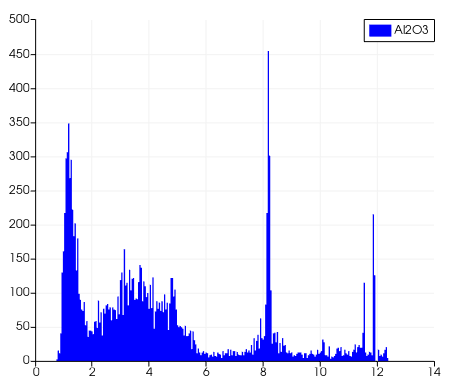
Fig. 3.16 A Histogram showing the Al2O3 attribute of a data table.¶

The Display panel allows to finetune the properties of the Histogram View as shown in Fig. 3.17.

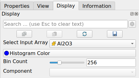
../_images/histogramview_displayproperties.png

Fig. 3.17 In the Display panel of the Histogram View, an attribute for the display can be selected and other display settings.¶

On top of that, additional properties regarding the X and Y axis of the Histogram View can be adapted in the View panel as shown in Fig. 3.18.

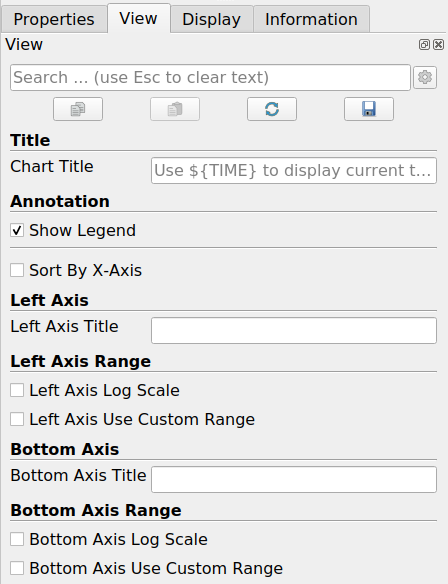
../_images/histogramview_viewproperties.png

Fig. 3.18 In the View panel, properties regarding the axes and chart titles can ge adapted.¶

Hint

The View Properties of a Histogram View are initially set in such a way that all the data are displayed, and they can be adapted in the View Panel as shown in Fig. 3.18. On top of that, the numeric display range can also be directly adapted with the mouse in the Histogram View display.

Such a histogram of the distribution of chemical compounds in a rock volume will give valuable insights about homogeneity or heterogeneity and other characteristics of of the materials.

3.3.2. Box Charts¶

Box Charts are a useful way for the visualization of more than one attribute - see Fig. 3.19.

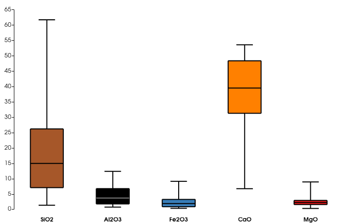
Fig. 3.19 Box chart example.¶

Generate a box chart by applying the Compute Quartiles filter to a block model, sampling set, drillhole data or all kinds of data tables.

3.3.3. Matrix of Correlation Charts¶

An even more powerful way to analyze the composition of rocks within a rock volume that is represented by a block model is the matrix of charts that can be displayed with the Plot Matrix View as shown in Fig. 3.20.

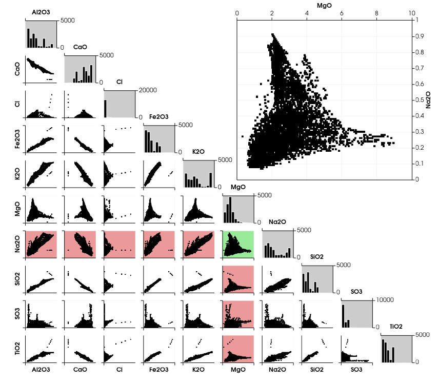
Fig. 3.20 The Plot Matrix View shows a matrix of charts¶

The following charts are shown in a Plot Matrix View:

a diagonal of histograms for all the selected chemical compounds.
in the lower left triangle, correlation diagrams for all chemical compounds with all others.
in the upper left triangle, one enlarged correlation diagram that can be selected from the lower left diagrams with a mouse click.

Select the chemical compounds to be included in the chart in the Display properties panel as shown in Fig. 3.21.

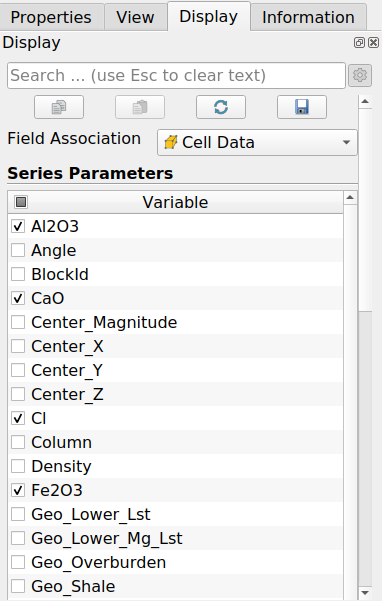
../_images/plotmatrixview_displayproperties.png

Fig. 3.21 In the Display properties panel, choose the compounds that should be included in the plots¶

Did you know?

With the little camera button above the upper left corner of the charts it is possible to copy the displayed chart directly into the clipboard for insertion into a report or other document. Pressing that button together with Ctrl, Alt or Shift will open a file dialog that allows to save the chart into an image file.

Did you know?

Chart display can be part of interesting linked selections, in two ways:

automatically updated chart display on changing data items or selections in other views
selecting items in a chart and automatically visualize them in a 3D (Render) or Table view

For more about selections see Selections.

3.4. Conclusion¶

The above examples for data display and analysis with AthosGEO View do not cover all the possibilities that are available thanks to the fact that the software is built on top of ParaView. For more information, follow the links that can be found here in First Steps.