4. Display a Topo
Most of what a user needs to know about display of a topo is already explained in Section 7:
File types (*.vtp, *.dxf and GeoTIFF files) and VTK data types (polydata for both triangulated surfaces or polylines/polygons).
Manually generating surfaces and polylines.
Simplification of triangulated surfaces and polylines with the Decimate and the Decimate Polyline filters.
Projection of a georeferenced bitmap image on a topo (with either ESRI World Files or GeoTIFF).
This section will show a few more ways how to display and manipulate topography data - basically triangulated surfaces.
4.1. Color by Elevation
A plain triangulated surface does not have attributes, so coloring by attribute is not possible, but this can easily be changed as follows:
Use the Calculator filter to generate an Elevation point attribute The formula would simply be coordsZ. This formula basically transfers the Z coordinate of the points to a new attribute that can be used for a color mapping display.
Now it is possible to color the surface by Elevation, as shown in Fig. 4.22.
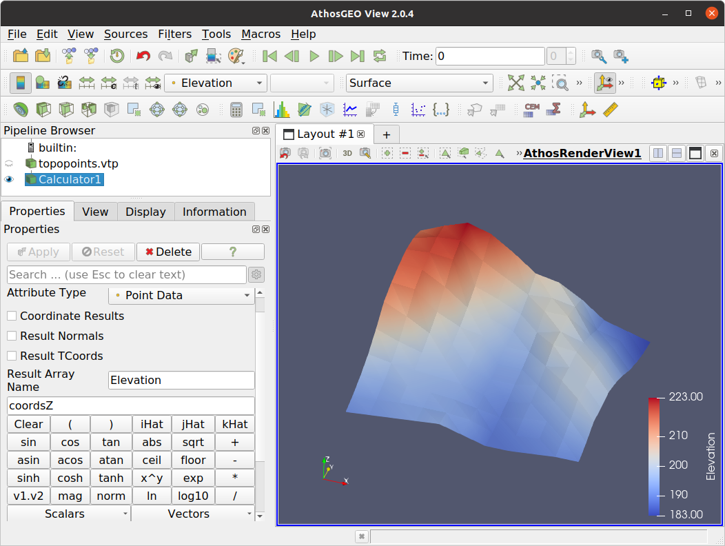
Fig. 4.22 Coloring a triangulated topo surface by a newly generated Elevation attribute.
Did you know?
As can be seen in Fig. 4.22, coloring appears nicely and smoothly interpolated. This is because the Elevation attribute is a Point attribute. See also Section 4.3 for more information about point and cell attributes.
4.2. Contour Lines
Once a triangulated surface has an Elevation point attribute as explained in Section 4.1, it is also possible to calculate contour lines for the topo surface with the Contour filter.
On the Properties panel, the elevations are defined in the Isosurfaces section. The result will be as shown in Fig. 4.23.
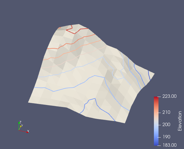
Fig. 4.23 Calculated contour lines for a triangulated topo surface. The lines are colored with the Elevation attribute, and the line width is increased in the Display panel to enhance visibility. The topo surface is shown as well, but could be turned off in the Pipeline Browser.
4.3. Point and Cell Attributes
While for block models and sampling sets it is clear that we are interested in cell attributes only, it makes a lot of sense for triangulated surfaces to care about both point and cell attributes, depending on the visual effect that is intended:
Point attributes are interpolated between the points, which results in smooth color transitions between the points, as shown in Fig. 4.22.
Cell attributes will result in a precise coloring where each triangle receives the color that corresponds to it’s cell attribute, with hard edges, as shown in Fig. 4.24.
Two filters are available for converting between point and cell attributes:
Point Data to Cell Data does what the name is saying: It converts point attributes into cell attributes. It does so by averaging all available point attributes of those points that are part of a specific cell. A result of applying this to the Elevations attribute that was generated in the previous section looks like shown in Fig. 4.24.
Cell Data to Point Data is doing the inverse operation of the previous filter. Also in this case, attribute values are averaged from adjoining cells.
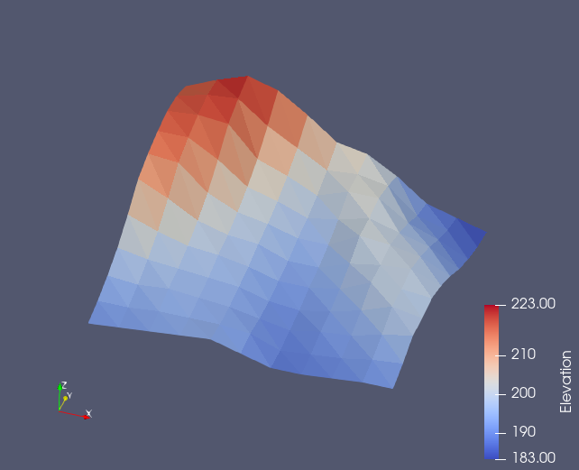
Fig. 4.24 Triangles are colored according to the average elevation of their adjoining points.
4.4. Direct Coloring
So far and by default, coloring is for an attribute by color mapping. However, it is possible to turn color mapping off and use color values that are directly stored as attributes:
In the following, Colors will be used as the attribute name for colors, but actually the name is unimportant: It is only the Map Scalars property that counts - see Fig. 4.25.
If a Colors attribute has one component, the values will be interpreted as grey values. If it has three components, the components will be interpreted as red, green and blue components.
If the data type of the Colors attribute is floating point values (float or double), the value range is between 0.0 and 1.0. If it is integer values, the value range would be 0 to 255.
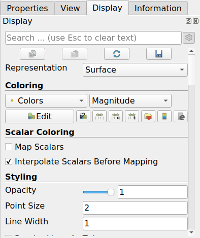
Fig. 4.25 The Map Scalars property is responsible for deciding whether attribute values are interpreted as colors directly (off) or colored via a color map (on, which is default) that can be manipulated with the Color Map Editor. Please note that below this property you find also the Opacity property that allows to make a surface semi-transparent.
In Fig. 4.26 you find an example where a full color (RGB) attribute is generated with the Calculator filter. However, it is completely irrelevant how that attribute is generated, as long as the conditions given above are followed.
In the example, the following formula is used to generate a Colors attribute:
iHat*(coordsX-10200)/100+jHat*(coordsY-24300)/100+kHat
Some explanatory hints about this formula:
iHat, jHat and kHat are actually the unity vectors (1,0.0), (0,1,0) and (0,0,1), so by multiplying with them, we are generating a 3-component attribute, not a single scalar only.
From coordsX we are subtracting 10200, which is the minimum X coordinate in the example, and we divide the result by 100, which is the value range of X. The same is true for the Y coordinate, and Z we ignore in this case.
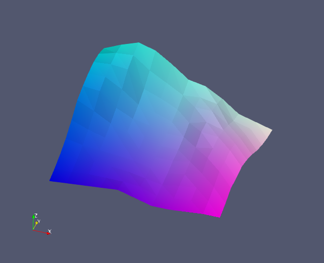
Fig. 4.26 In this example, coloring is the more red (or magenta) the higher the X coordinate, green is increasing with the Y coordinate, and where both are small, blue becomes the dominating color.
Another example is shown in Fig. 4.27 that shows an explicit example for greyscale coloring by elevation.
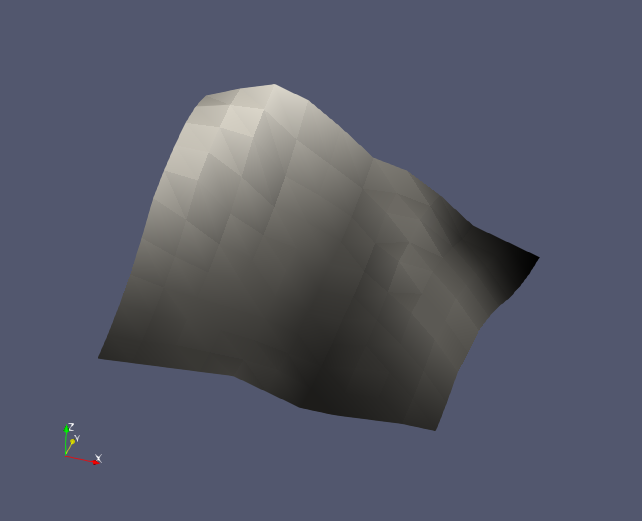
Fig. 4.27 Here greyscale coloring is directly from a one-component attribute with values going from 0.0 to 1.0.
4.5. Write Value and Write Multiple Values for Surfaces or Polylines
The Write Value and the Write Multiple Values filters are described in the sections Write Value and Write Multiple Values , both for a block models, but they can be equally well applied to triangulated surfaces or polylines where it will affect the Cell attributes of the triangles or line segments, respectively, as shown in Fig. 4.28, with results as shown in Fig. 4.29.
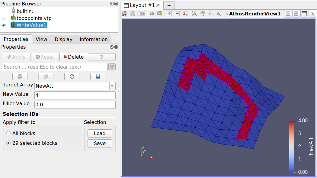
Fig. 4.28 The Write Value filter allows to “paint” values on a triangulated topo surface
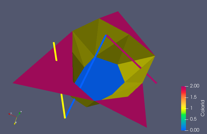
Fig. 4.29 Example with a triangulated surface and a polyline that are colored by their assigned attributes
Note
In the same way as with the Write Value filter, also the Calculator, the Calculator for Selection and the Write Multi Values filters can be applied to triangulated topo surfaces: see Section 4, where they are all explained for block models.
Hint
If the resolution of the triangle grid is too coarse grained for the assignment of a specific coloring, it can be refined using the Subdivide filter.
4.6. LAS (Laser Scanner) File Reader
AthosGEO View has a reader for laser scanner (LAS) files. The output is a point cloud which may have point attributes: see Fig. 4.30 for an example.
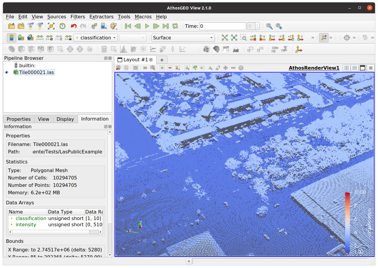
Fig. 4.30 Example of a point cloud from a laser scanner, with a classification attribute.
Hint
If the LAS data set has a colors attribute, it’s values will be adjusted in such a way that RGB color can be directly displayed by turning the Map Colors off in the Display panel.
Note
LAS files can be very large, and whether AthosGEO View will be able to process the data depends on the memory of the computer system. This is not only true for plain reading and display: system overload can also happen if any filters are applied.